We are currently using AWS OpenSearch Service as a vector store for our RAG with AWS Bedrock Knowledge Base.

We will talk more about RAG and Bedrock another time, but today let’s take a look at AWS OpenSearch Service.

The task is to migrate our AWS OpenSearch Service Serverless to Managed, primarily due to (surprise) cost issues – because with Serverless, we constantly have unexpected spikes in OpenSearch Compute Units (OCU – processor, memory, and disk) usage, even when there are no changes in the data.

The main task is to plan the cluster size: disks, CPU and memory, and select the appropriate instance types.

In the second part, we will talk about access settings – AWS: creating an OpenSearch Service cluster and setting up authentication and authorization.

Elasticsearch vs OpenSearch vs AWS OpenSearch Service

In fact, OpenSearch is essentially the same as Elasticsearch: when Elasticsearch changed its license terms in 2021, AWS launched its own fork, naming it OpenSearch.

OpenSearch is compatible with Elasticsearch up to version 7.10, but unlike Elasticsearch, OpenSearch has a completely free license.

I once wrote about launching Elasticsearch as part of the ELK stack for logs here – Elastic Stack: overview and installation of ELK on Ubuntu (2022), but that article is more about self-hosted solutions and working with indexes in general. Now we will look specifically at the solution from AWS.

AWS OpenSearch Service is a fully AWS-managed service: as with Kubernetes, AWS takes care of all deployment, updates, and backups, and has tight integration with other AWS services – IAM, VPC, S3, and Bedrock, which is what we use it with.

AWS OpenSearch Service: an intro

Here and below, I will mainly talk about the Managed OpenSearch Service.

The basic concepts of AWS OpenSearch Service are domains, nodes, indexes (“databases”), and shards.

A “domain” is the cluster itself, which we configure to the desired number and type of nodes, and indexes are divided into shards (data blocks) that are distributed among the nodes:

The nodes in the cluster are essentially regular EC2 instances (as in RDS or even AWS Load Balancer), where the same regular compute instances run under the hood.

For the AWS OpenSearch Service cluster, as with Elastic Kubernetes Service, separate control nodes (master nodes) are created, but unlike EKS, we do not need to manage the Data Plane and WorkerNodes separately here.

As with RDS, we can set up automatic backups for the OpenSearch cluster.

For data visualization, AWS provides OpenSearch Dashboards.

Data schema: documents, indexes, and shards

To understand what types of instances to choose for our cluster, let’s take a look at what indexes are in OpenSearch (or Elasticsearch, because they are essentially the same thing).

So, an index is a collection of documents that have some common features. Each index has a unique name, just like a database in RDS PostgreSQL or MariaDB.

Although an index is often compared to a database, in practice it is more convenient to think of an index as a table, and the “database” as the entire cluster.

A document is a JSON object in an index and represents a basic unit of data storage. If we draw an analogy with the SQL databases, it is like a row in a table.

Each document has a set of key-value fields, where values can be strings, integers, dates, or more complex structures such as arrays or objects.

Indexes are divided into parts called shards for better performance, where each shard contains a portion of the index data. Each document is stored in only one shard, and searches can be performed in parallel across multiple shards.

Although technically not entirely accurate, shards can be thought of as separate mini-indexes or mini-databases.

Shards can be primary or replica: primary accepts all write operations and can process select, while replica is only for read-only operations.

At the same time, a replica is always created on another data node for fault tolerance, and a replica can become primary if the node with the primary shard fails.

The default value for the number of shards per index in AWS OpenSearch Service is 5, but it can be configured separately (i.e., with 5 primary shards, we will have 10 shards in total, because there will also be replicas).

It is recommended that shards be between 10 and 50 gigabytes in size: each shard requires CPU and memory to work with it, so a large number of small shards will increase the need for resources, while shards that are too large will slow down operations on them.

In the open-source OpenSearch (and Elasticsearch), the default number of primary shards is 1.

New documents are distributed evenly among all available shards.

Amazon OpenSearch Service 101: How many shards do I need

Data, Master, and Coordinator Nodes

Data Nodes – store data and shards, and execute search and aggregation queries. These are the main “working units” of the cluster.

Master Nodes – store metadata about indexes, mapping, cluster status, manage primary/replica shards, perform rebalancing – but do not process search queries. That is, their task is exclusively to control the cluster.

Coordinator nodes (client nodes) do not store any data and do not participate in its processing. The role of these nodes is to act as a kind of “proxy” between the client and the data nodes. They receive a query from the client, divide it into subqueries (scattering), send them to the appropriate data nodes, then collect the result (gather) and return it to the client. However, it is advisable to have separate nodes under Coordinators on large clusters in order to reduce the load on Master and Data nodes.

Pricing

As with most similar AWS services, we pay for compute resources (CPU, RAM) per disk (EBS) and for traffic – although traffic has some nuances (for the better) – because for multi-AZ deployments, we don’t pay for traffic between nodes in different Availability Zones (in RDS, too, I think), nor do we pay for traffic between UltraWarm/Cold Nodes and AWS S3.

Full documentation on pricing is available at Amazon OpenSearch Service Pricing, and here are the main points:

t3.medium.search: 2 vCPU, 4 GB RAM – $0.073 (regular t3.medium EC2 will cost less – $0.044)
General Purpose SSD (gp3) EBS: $0.122 per GB/month (regular EBS for EC2 – $0.08/GB-month)

Similar to AWS EKS, OpenSearch Service has two types of update support – Standard and extended – and, of course, Extended will be more expensive.

Hot, UltraWarm, and Cold storage in the OpenSearch Service

Data (indexes) storage in OpenSearch Service can be organized either on EBS on the data node itself (Hot), cached on a node with a “backend” in S3 (UltraWarm), or only in S3 (Cold):

Hot storage: regular data nodes on regular EC2 with EBS – for the most relevant data, provides fast access to data
UltraWarm storage: for data that is still relevant but not frequently accessed – data is stored in S3, and their cache is stored on the nodes, with the nodes themselves being a separate type of instance, such as ultrawarm1.medium.search
- fast access to data that is in the cache, slower access to data that has not been accessed for a long time
- the nodes themselves are more expensive (ultrawarm1.medium.search will cost $0.238), but savings are achieved by storing data in S3 instead of EBS
- read-only data
- not available whether there are T2 or T3 instances in the cluster 🙁
Cold storage: this data is stored exclusively in S3 and can be accessed via the OpenSearch Service API
- slow access, but here we only pay for S3
- to use it, you need to have the Warm storage configured
- similarly, not available if there are T2 or T3 instances in the cluster 🙁

This is well described in Choose the right storage tier for your needs in Amazon OpenSearch Service.

Automatic backups are free and stored for 14 days.

Manual backups are charged for S3 storage, but there is no charge for the traffic used to store them.

Planning an AWS OpenSearch Service domain

OK, now that we’ve covered the basics, let’s think about how we’re going to build the cluster – its capacity planning and the selection of instance types for Data Nodes.

Storage

Choosing the size of disks

A very important point to start with is to determine how much space your index or indexes will take up.

This is well described in the Calculating storage requirements documentation, but let’s calculate it ourselves.

For example, we will have 3 data nodes, and we will store some logs.

We record 10 GiB of logs per day, which we store for 30 days, resulting in 300 gigabytes of occupied space. With three nodes, that’s 100 gigabytes per node.

But we also need to consider the following:

Number of replicas: each replica shard is a copy of the primary shard, so it will take up about the same amount of space
OpenSearch indexing overhead: OpenSearch takes up additional space for its own indexes; this is another +10% of the size of the data itself
Operating system reserved space: 5% of space on EBS is reserved by the operating system
OpenSearch Service overhead: another 20% – but no more than 20 gigabytes – is reserved on each node by OpenSearch Service itself for its own work

The documentation provides an interesting clarification on the last point:

if we have 3 nodes, each with a 500 GB disk, then together we will have 1.5 terabytes, while the total maximum amount of space reserved for OpenSearch will be 60 GB – 20 GB for each node
if we have 10 nodes, each with a 100 GB disk, then together we will have 1 terabyte, but the maximum amount of space reserved for OpenSearch will be 200 GB – 20 per node.

The formula for calculating space looks like this:

Source data * (1 + number of replicas) * (1 + indexing overhead) / (1 - Linux reserved space) / (1 - OpenSearch Service overhead) = minimum storage requirement

That is, if we need to store 300 GB of logs, we calculate:

Source data: 300 GiB
1 primary + 1 replica
1 + indexing overhead = 1.1 (+10% of 1)
1 – Linux reserved space = 0.95 (5%)
1 – OpenSearch Service overhead = 0.8 (but this is true if the disks are less than 100 GB)

In this case, for our 300 GiB of logs, we need:

300*2*1.1/0.95/0.8
867

867 GiB of total space.

Or there is a simpler formula – just use a coefficient of 1.45:

Source data * (1 + number of replicas) * 1.45 = minimum storage requirement

Then it turns out:

300*2*1.45
870.00

Almost the same 867 gigabytes.

Number of shards

The second important point, which is also described in the documentation, is Choosing the number of shards.

The essence is that in AWS OpenSearch Service, the index is split into 5 primary shards without replicas by default (in self-hosted Elasticsearch/OpenSearch, the default is 1 primary and 1 replica).

Once the index is created, you cannot simply change the number of shards, because the routing of requests to documents is tied to specific shards (this is well described here: Distributing Documents across Shards (Routing)).

The recommended shard size is 10-30 GiB for data with more searches and 30-50 for indexes with more write operations.

Indexing overhead, which we mentioned above, must be added to the size of the index itself – 10%.

If we consider a case where we write logs (i.e., write-intensive workload), the maximum index size will be 300 GiB + 10% == 330 GiB.

If we want to have primary shards of, say, 30 gigabytes, we get 11 primary shards.

Changing the number of primary shards requires creating a new index and performing a reindex – copying data from the old index to the new one, see Optimize OpenSearch index shard sizes.

But!

If the index is planned to be small, it is better to have one shard + 1 replica; otherwise, the cluster will create unnecessary empty shards that still consume resources.

In this case, it is still recommended to have three nodes: one will be the primary shard, the second will be the replica, and the third will be the backup:

if node-1 with the primary fails, node-2 will make the replica the new primary
and node-3 will receive a new replica

Choosing a type of Data Nodes

Another important point is how to choose the right type of data node.

What we need to understand in order to choose a node are the CPU, RAM, and disk requirements.

The documentation Choosing instance types and testing states:

try starting with a configuration closer to 2 vCPU cores and 8 GiB of memory for every 100 GiB of your storage requirement

But this is just for “starting”, and it is recommended to run some load tests and monitor the results.

We will talk about monitoring separately, but for now, let’s try to make our own estimate for the hardware we need.

Another useful resource is here: Operational best practices for Amazon OpenSearch Service.

Instance types

See Supported instance types in Amazon OpenSearch Service and Amazon OpenSearch Service Pricing.

The general rules here are the same as for regular EC2:

General Purpose (t3, m7g, m7i): standard servers with balanced CPU/RAM
- well suited for master nodes or data nodes on small clusters
Compute Optimized (c7g, c7i): more CPU, less memory
- suitable for data nodes that need more CPU (indexing, complex searches, and aggregations)
Memory Optimized (r7g, r7gd, r7i): conversely, more memory, less CPU
- suitable for data nodes that need more RAM
Storage Optimized (i4g, i4i): better SSDs (NVMe SSDs) with high IOPS
- suitable for data nodes that need to perform many write operations (logs, metrics)
OpenSearch Optimized (om2, or2): “tuned” instances from AWS itself with an optimal CPU/RAM ratio and disks, easier to configure
- this is something for rich and large clusters 🙂

Indexes here:

g: Gravitor processors (ARM64 from AWS) – productive for multi-threaded computations, better in terms of price:performance, but there may be compatibility issues
i: Intel (based on x86 – classic, compatible with everything, better for heavy single-threaded computations
d: “drive” – has an additional NVMe SSD

Data Node Storage

We seem to have figured out the disk in Choosing the number of shards:

10-30 gigabytes per shard if we plan to have more search operations
30-50 GiB per shard if there are more write operations

Next, we select the instance type so that it has enough storage, because there is still a limit on disk size – see EBS volume size quotas.

Data Node CPU

In the Shard to CPU ratio section, there is a recommendation to plan for “1.5 vCPU per shard”.

That is, if we plan to have 4 shards per data node, we allocate 6 vCPUs. We can add 1 (preferably 2) more cores for the needs of the operating system itself.

However, again, a lot depends on how the data will be processed.

If there are many search-heavy operations, then 1.5 CPU per shard is quite justified.

For write-intensive operations, you can consider 0.5 CPU per shard, and for warm and cold nodes, even less.

See OpenSearch Threadpool.

Data Node RAM

Now for the most interesting part: how do we calculate the required memory?

Here, the calculations will depend heavily on the type of index and data – whether it is simply documents in the form of logs or, as in our case, a vector store.

Before we calculate the requirements, let’s take a quick look at how memory is distributed on the instance:

JVM Heap Size: by default, it is set to 50% of RAM (but no more than 32 gigabytes): in the JVM Heap, we will have various OpenSearch proprietary data – metadata and shard/index management (mappings, routing, cluster status), query and response objects, search coordination, various internal caches and buffers – that is, purely internal needs of OpenSearch itself
off-heap memory (the operating system’s own memory):
- when using the index as a vector store – HNSW graphs (k-NN search) + Linux page cache for data that is loaded from disk into OS memory for fast access
- for simple logs – only Linux page cache for data that is loaded from disk into OS memory

Calculating RAM for logs

We plan to allocate 16 gigabytes for the JVM heap, keeping in mind that this will be 50%. Alternatively, we could allocate at least 8 gigabytes and then monitor JVMMemoryPressure (we will speak about monitoring more in a following blog post, it’s already in drafts).

Next, we estimate the memory under off-heap – Linux will do mmap relevant for processing data requests (read data blocks from disk into memory when the process requests them).

Here we will have the “hot data” – that is, the data that is often needed by clients. For example, we know that most often we will be searching the logs for the last 24 hours, and we write 10 gigabytes of logs per day.

To these 10 GB, we should add 10-50 percent for the OpenSearch structures themselves, so the index will grow by 11-15 GB per day.

Of these 11-12 gigabytes, let’s say 50% will be actively used for search results – we’ll allocate 5-6 GiB of RAM for the “hot OS page cache”.

RAM calculation for vector store

If we use OpenSearch as a vector database, we need to consider the memory requirements for each graph for data search.

The size of the graph depends on the algorithm, but let’s take the default one – HNSW (Hierarchical Navigable Small Worlds). The choice of algorithm is well described in Choose the k-NN algorithm for your billion-scale use case with OpenSearch.

In order to estimate how much memory the HNSW structure will take up, we need to know the number of vectors in the index, their dimension (embedding dimension), and the number of connections between each node in the graph (how many neighbors to store for each point in this graph).

What do we have in the “vector” anyway?

a set of numbers specified in the dimension embedding model ([0.12, -0.88, ...])
metadata: various key:value pairs with information about which document this vector belongs to, source, and so on
optionally – the original text itself (the _source field does not affect the graph, but increases the size of the index)

id: "doc1-chunk1"
knn_vector: [0.12, -0.33, ...]   // number set by dimension parameter
metadata: {doc_id: "doc1", chunk: 1, text: "some text"}

RAG, AWS Bedrock Knowledge Base, data, and vector creation

The RAG process itself is well described in this diagram (see Implementing Amazon Bedrock Knowledge Bases in support of GDPR (right to be forgotten) requests):

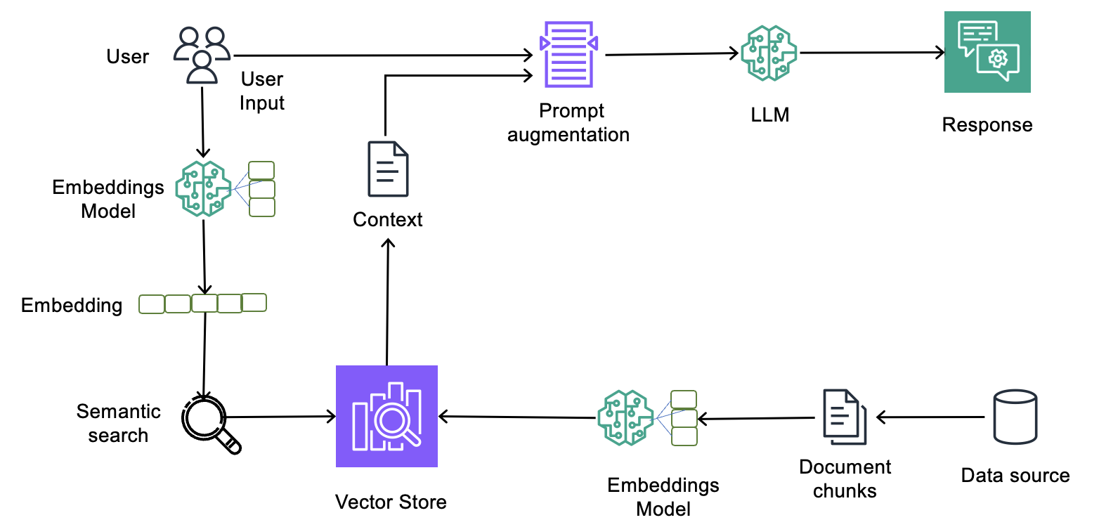
Here is an overview of how RAG works and the role of the vector database in it:

The client (e.g., a mobile app) sends a request to our Backend API, which runs on Kubernetes.
The Backend API receives it and generates a RetrieveAndGenerate request to Bedrock, which transmits the Knowledge Base ID and the text of the client’s request
Bedrock launches the RAG pipeline, in which:
- it sends a request to the embedding model to convert it into a vector (s)
- performs a k-NN search in the OpenSearch index to find the most relevant data
- forms an extended prompt that contains the original request + the data returned by OpenSearch
- calls the GenAI model, to which it passes this extended prompt
- receives a response from it
- returns it in JSON format to our Backend API
The Backend API sends the result to the client

How the process of converting text to vectors looks like in AWS Bedrock Knowledge Base:

We have some source – for example, a txt file in S3
Bedrock reads it, and if it is large, it divides it into chunks with a size specified in the Bedrock parameters
Bedrock sends each chunk of text to the embedding LLM model, which converts this chunk into a vector of fixed length (dimension) and returns it to the Bedrock pipeline
Bedrock sends this vector along with metadata to the AWS OpenSearch vector store, where it is indexed for k-NN search

Number of vectors

The number of vectors in the index primarily depends on the data corpus (the size of all the input data we are working with) and how many chunks they will be divided into.

What you need to understand: vectors are not created for individual tokens, but for parts of text, for whole phrases.

Each embedding model has a limit on the number of tokens it can process at a time (the maximum “input length”).

If the text is long, it is broken down into chunks, and a separate vector is created for each chunk.

If we take, for example, an embedding model with a limit of 512 tokens and a dimension (dimension, d) of 1024 numbers, then:

the phrase “hello, world” fits into one “window” for embedding, and 1 vector will be created
a 300-word paragraph of English text will yield approximately 400 tokens – this also fits into the window, and 1 embedding vector will also be created
an article of 1,000 words will give approximately 1,300-1,400 tokens, so it will be divided into three chunks, and separate vectors will be created for them:
- chunk_1 => [vector_1 with 1024 numbers]
- chunk_2 => [vector_2 with 1024 numbers]
- chunk_3 => [vector_3 with 1024 numbers]

d (dimension): is set by the embedding model, which converts data into vectors for storage in the vector store. For example, in Amazon Titan Embeddings, dimension=1024. This same parameter is specified when creating an index.

m (Maximum number of bi-directional links): the number of links between each node in the graph, this is a parameter of the HNSW graph, specified when we create an index, for example:

"bedrock-knowledge-base-default-vector": {
  "type": "knn_vector",
  "dimension": 1024,
  "method": {
    "name": "hnsw",
    "engine": "faiss",
    "parameters": {
      "m": 16,
      "ef_construction": 512
    },
    "space_type": "l2"
  }
}

Now, knowing all this data, we can calculate how much memory will be needed to build the graph in memory, for example:

a number of vectors: 1,000,000
d=1024
m=16

Formula:

num_vectors * 1.1 * (4 * d + 8 * m)

Here:

1.1: 10% reserve is added for HNSW service structures
4: each coordinate (number in the vector) is stored as float32 = 4 bytes
8: number of bytes for storing the id of each “neighbor” (64-bit int) (the number of which is given by m)

So, let’s calculate:

1.000.000 * 1.1 * (4*1024 + 8*16)

4646400000.0 bytes, or 4.64 gigabytes, is the volume for the HNSW graph across all vectors (excluding replicas and shards, which will be discussed later).

Now let’s consider the distribution into chunks and data nodes:

if we have a total index of 100 gigabytes
divided into 3 primary shards, and for each primary we have 1 replica shard – a total of 6 shards
we have 3 data nodes – each node will have 2 shards

A separate graph will be built for each shard, so we multiply 4.64 gigabytes by 2.

But since the index is distributed across 3 nodes, we divide the result by 3.

So the calculation will be as follows:

graph_total: our 4.64 gigabytes, the total volume for the graph
graph_cluster: graph_total * (1 + replicas) (primary + all replicas)
graph_per_node = graph_cluster / number of data nodes in the cluster

The formula will be as follows:

graph_total * (1 + replicas) / num_data_nodes

Having 1 primary shard + 1 replica shard, we get:

4.64 gigabytes * 2 / 3 data nodes

~ 3.1 GiB of memory per node purely for graphs.

k-NN graphs are stored in off-heap memory, so we can already estimate:

8 (preferably 16) gigabytes under JVM Heap for OpenSearch itself
3 GiB under graphs

The limit for k-NN graphs is set in knn.memory.circuit_breaker.limit, and is usually 50: off-heap memory – see k-NN differences, tuning, and limitations.

The metric in CloudWatch is KNNGraphMemoryUsage, see k-NN metrics.

Or in the OpenSearch API itself – _plugins/_knn/stats and _nodes/stats/indices,os,break (see Nodes Stats API).

And to this we must add the OS page cache for “hot” data – vectors/metadata/text that are mapped from disk to memory for quick access – as we calculated for the index with logs.

For the OS page cache, we can add another 20-50% of the total index size on the node, although this depends on the operations that will be performed. Ideally, if money is no object, you can add another 100% of the index size * 2 (for each replica of each shard) / number of nodes.

So, if we take 1,000,000 vectors in the database, and the database itself is 30 gigabytes, 3 primary shards and 1 replica for each, and 3 data nodes, we get: